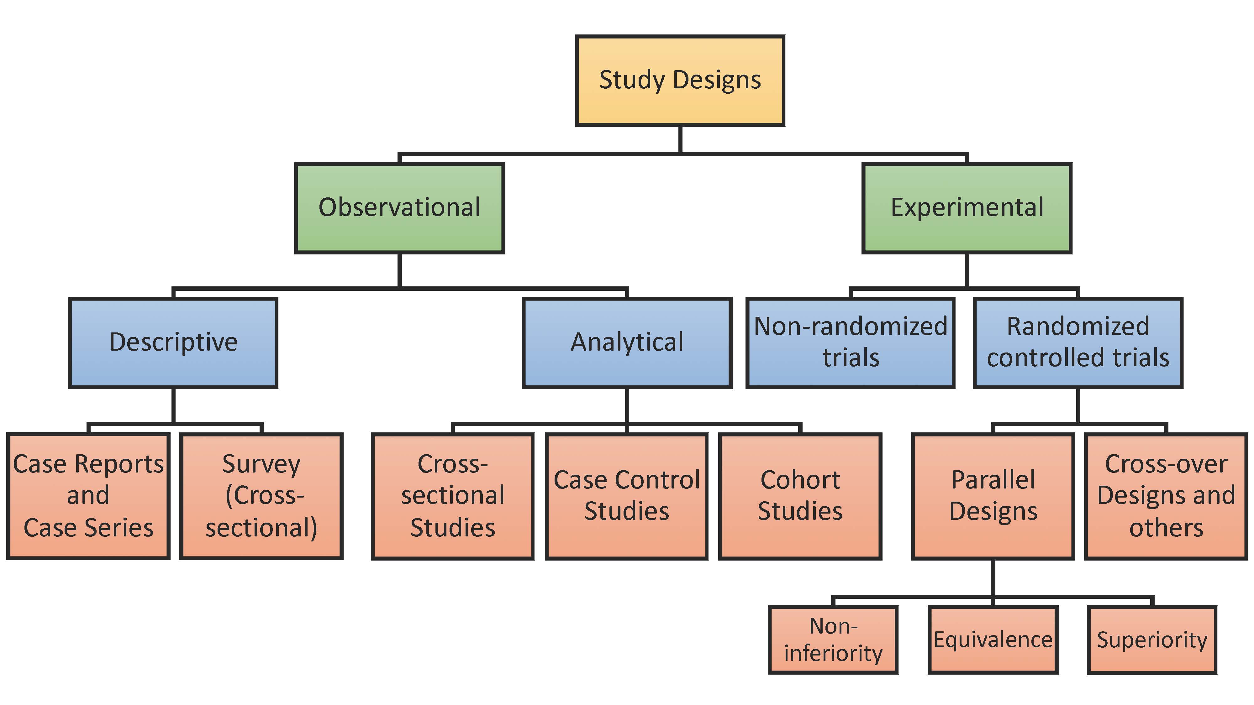
Introduction Select your clinical design Randomized Control Trial (Parallel) Non-inferiority Trial Equivalence Trial Superiority Trial Observational Study Cohort Study Case-control Study Cross-sectional Study Survey (Cross-sectional) Prediction Model Prediction Model Area under ROC curve

Chow S-C, Shao J, Wang H, Lokhnygina Y. Sample Size Calculations in Clinical Research. Third ed: Chapman and Hall/CRC; 2017.
Type I error rate, \(\alpha\)
Ratio of case to control, \(k\)
Allowable difference, \(d=\mu_T-\mu_C\)
Expected population standard deviation, \(\text\)
Drop rate (%, 0 ~ 99)
Chow S-C, Shao J, Wang H, Lokhnygina Y. Sample Size Calculations in Clinical Research. Third ed: Chapman and Hall/CRC; 2017.
Type I error rate, \(\alpha\)
Ratio of case to control, \(k\)
Drop rate (%, 0 ~ 99)
Proportion Odds ratioMargin on risk difference scale (\(\delta \geq 0)\)
Margin for log-scale odds ratio (\(\delta>0)\)
Schoenfeld D. The Asymptotic Properties of Nonparametric-Tests for Comparing Survival Distributions. Biometrika. 1981;68(1):316-319.
Schoenfeld D. Sample-Size Formula for the Proportional-Hazards Regression-Model. Biometrics. 1983;39(2):499-503.
Type I error rate, \(\alpha\)
Ratio of case to control, \(k\)
Margin for log-scale hazard ratio (\(\delta\)>0)
Known probabilities of event during the trial Estimate probabilities of event during the trial using exponential modelAccrual time period, \(T_a\)
Follow-up time period, \(T_b\)
Hazard for the control group , \(\lambda_C\)
Fleiss JL, Levin B, Paik MC. Statistical Methods for Rates and Proportions. Third ed: John Wiley & Sons; 2013.
A case-control study of the relationship between smoking and CHD is planned. A sample of men with newly diagnosed CHD will be compared for smoking status with a sample of controls. Assuming an equal number of cases and controls (i.e., \(k = 1\)). Previous surveys have shown that around 0.40 of males without CHD are smokers (i.e., \(p_0 = 0.4\)). For achieving an 90% power (i.e., \(1-\beta = 0.9\)) at the 5% level of significance (i.e., \(\alpha = 0.05\)), the sample size to detect an odds ratio of 1.5 (i.e., \(OR = 1.5\) or \(p_1 = 0.5\)) is \(519\) cases and \(519\) controls or \(538\) cases and \(538\) controls by incorporating the continuity correction.
Two-sided (Unchecking the checkbox will perform the sample estimation for a one-sided test.)Type I error rate, \(\alpha\)
Ratio of case to control, \(k\)
Proportion Odds ratioDupont WD. Power calculations for matched case-control studies. Biometrics. 1988;44(4):1157-1168.
Suppose a researcher conduct a matched case-control study to assess whether bladder cancer may be associated with past exposure to cigarette smoking. Cases will be patients with bladder cancer and controls will be patients hospitalised for injury. One case will be matched to one control (i.e., \(k = 1\))and the correlation between case and control exposures for matched pairs is estimated to be 0.01 (low, i.e., \(r = 0.01\)). It is assumed that 20% of controls will be smokers or past smokers (i.e., \(p_0 = 0.2\)), and the researcher wish to detect an odds ratio of 2 (i.e., \(OR = 2\) or \(p_1 = 0.67\)) with power 90% (i.e., \(1-\beta = 0.9\)). The sample size needed for cases and controls is \(16\) and \(16\), respectively.
Two-sided (Unchecking the checkbox will perform the sample estimation for a one-sided test.)Type I error rate, \(\alpha\)
Ratio of case to control, \(k\)
Proportion Odds ratioWoodward M. Formulae for sample size, power and minimum detectable relative risk in medical studies. Journal of the Royal Statistical Society: Series D (The Statistician). 1992;41(2):185-196.
Fleiss JL, Tytun A, Ury HK. A simple approximation for calculating sample sizes for comparing independent proportions. Biometrics. 1980;36(2):343-346.
A government initiative has decided to reduce the prevalence of male smoking to 30% (i.e., \(p_1 = 0.3\)). A sample survey is planned to test, at the 0.05 level (i.e., \(\alpha = 0.05\)), the hypothesis that the percentage of smokers in the male population is 30% against the one-sided alternative that it is greater. The survey should be able to find a prevalence of 32% (i.e., \(p_0 = 0.32\)), when it is true, with 0.90 power (i.e., \(1-\beta=0.9\)). The survey needs to sample \(9158\) in males pre inititative and \(9158\) in males post government initiative (or \(9257\) and \(9257\) by incorporating the continuity correction).
Two-sided (Unchecking the checkbox will perform the sample estimation for a one-sided test.)Type I error rate, \(\alpha\)
Drop rate (%, 0 ~ 99)
Ratio of unexposed to exposed, \(k\)
Proportion Relative riskChow S-C, Shao J, Wang H, Lokhnygina Y. Sample Size Calculations in Clinical Research. Third ed: Chapman and Hall/CRC; 2017.
Woodward M (2005). Epidemiology Study Design and Data Analysis. Chapman & Hall/CRC, New York, pp. 381 - 426.
Supposed we wish to test, at the 5% level of significance (i.e., \(\alpha = 0.05\)), the hypothesis that cholesterol means in a population are equal in two study years against the one-sided alternative that the mean is higher in the second of the two years. Suppose that equal sized samples will be taken in each year (i.e., \(k=1\)), but that these will not necessarily be from the same individuals (i.e. the two samples are drawn independently). Our test is to have a power of 0.95 (i.e., \(1-\beta = 0.95\)) at detecting a difference of 0.5 mmol/L (i.e., \(m_0 = 0, m_1 = 0.5\)). The standard deviation of serum cholesterol in humans is assumed to be 1.4 mmol/L (i.e., \(SD = 1.4\)). We need to test \(170\) in the first year and \(170\) in the second year.
Two-sided (Unchecking the checkbox will perform the sample estimation for a one-sided test.)Type I error rate, \(\alpha\)
Ratio of unexposed to exposed, \(k\)
Expected population standard deviation, \(\text\)
Breslow NE, Day NE, Heseltine E, Breslow NE. Statistical Methods in Cancer Research: The Design and Analysis of Cohort Studies. International Agency for Research on Cancer; 1987.
A matched cohort study is to be conduct to quantify the association between exposure A and an outcome B. Assume the prevalence of event in unexposed group is 0.60 (i.e., \(p_0 = 0.6\)) and the correlation between exposed and unexposed for matched pairs is 0.20 (moderate, i.e., \(r = 0.2\)). In order to detect a relative risk of 0.75 (i.e., \(RR=0.75\) or \(p_1 = 0.45\)) with 0.80 power (i.e., \(1-\beta = 0.8\)) using a two-sided 0.05 test (i.e., \(\alpha=0.05\)), there needs to be \(1543\) unexposed and \(1543\) exposed.
Two-sided (Unchecking the checkbox will perform the sample estimation for a one-sided test.)Type I error rate, \(\alpha\)
Drop rate (%, 0 ~ 99)
Proportion Relative riskSchoenfeld D. The Asymptotic Properties of Nonparametric-Tests for Comparing Survival Distributions. Biometrika. 1981;68(1):316-319.
Schoenfeld D. Sample-Size Formula for the Proportional-Hazards Regression-Model. Biometrics. 1983;39(2):499-503.
Rubinstein LV, Gail MH, Santner TJ. Planning the duration of a comparative clinical trial with loss to follow-up and a period of continued observation. J Chronic Dis. 1981;34(9-10):469-479.
Suppose a two-arm prospective cohort study with 1 year accrual time period (period of time that patients are entering the study, \(T_a = 1\)) and 1 year follow-up time period (period of time after accrual has ended before the final analysis is conducted, \(T_b=1\)). Assume the hazard for the unexposed group is a constant risk over time at 0.5 (i.e., \(\lambda_0 = 0.5\)). To achieve 80% power (i.e., \(1-\beta=0.8\)) to detect Hazard ratio of 2 (i.e., \(HR = 2\)) in the hazard of the exposed group by using a two-sided 0.05-level log-rank test (i.e., \(\alpha=0.05\)), the required sample size for unexposed group is \(53\) and for exposed group is \(53\).
Two-sided (Unchecking the checkbox will perform the sample estimation for a one-sided test.)Type I error rate, \(\alpha\)
Ratio of unexposed to exposed, \(k\)
Known probabilities of event during the trial Estimate probabilities of event during the trial using exponential modelAccrual time period, \(T_a\)
Follow-up time period, \(T_b\)
Hazard for the unexposed group , \(\lambda_0\)
Woodward M. Formulae for sample size, power and minimum detectable relative risk in medical studies. Journal of the Royal Statistical Society: Series D (The Statistician). 1992;41(2):185-196
Suppose that the primary interest lies in comparing systolic blood pressure between the two cities. Assume that simple random sampling from among 40-44-year-old men is to be used in each city with twice as many sampled from City 1 as from City 2, so that \(k=2\). Systolic blood pressure is to be compared using a one-sided 5% significance test (i.e. \(\alpha = 0.05\)). The medical investigators wish to be 95% sure of detecting when the average blood pressure in City 1 exceeds that in City 2 by 3 mm Hg (i.e., \(1-\beta=0.95\) and \(m_1 = 3\), \(m_2 = 0\)). From published literature (Smith et al. 1989) the standard deviation of systolic blood pressure is likely to be 15.6mmHg (i.e. \(SD=15.6\)). The sample size required is \(878\) for City 1 and \(439\) for City 2.